Must-Know Sorting Algorithms in Python

Your one-stop-shop for implementations of common sorting algorithms, written in Python. I strongly suggest having a basic knowledge of computing complexity and big oh notation before reading this post. If you’re new to the topics, I recommend MIT’s class 6.00.1x on edx.org. For convenience, here are links to the relevant lectures on YouTube: part 1 and part 2 (which overlaps somewhat with the concepts in this post specifically).

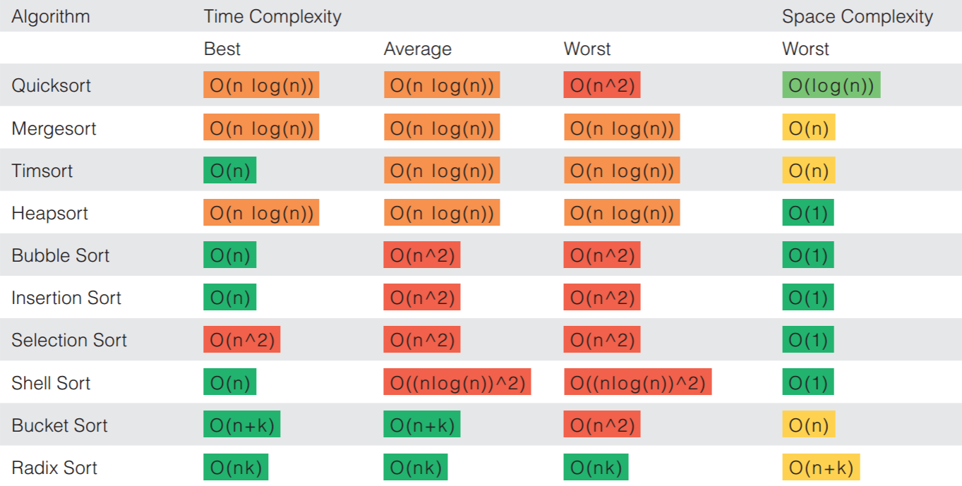
With that, we’ll dive right in, first with a quick table of the algorithms we’ll be discussing and their complexity:

As you can see, above, there are orders of magnitude differences in the efficiencies of some of the algorithms, and there seem to be more or less three “groups” of algorithms based on time complexity: “simple,” “efficient,” and “Distribution” sorts. In terms of operations, the first two categories will all be comparison-based algorithms (with sub categorizations of exchange, selection, insertion, and merge sorts), while distribution sorts are non-comparison-based. Don’t worry about these terms yet. I only introduce them here to give a high level overview of the topics presented below.

Note: As we walk through the code below, I will use a couple of short-hands, which are easier to explain once upfront. First, “L” will be out default variable name to represent a list to sort (not really consistent with Python naming conventions, but will make our code shorter). Secondly, I will use a technique for switching variable values without a temporary placeholder, so that we can rewrite

temp = x
x = y
y = temp

temp = x

x = y

y = temp

x, y = y, x

1	x, y = y, x

Simple Comparison-Based Sorts (Average O(n^2) time complexity)

Bubble Sort. Bubble sort is perhaps the most basic and in most cases least efficient sorting algorithm. It works by passing through a list, comparing two adjacent items at a time as it goes, and swapping those items in place to the correct order (our example will order from smallest to largest). Each pass will put at least one more item in its correct spot (more than one being correct is chance as opposed to design). The process is then repeated until no further swaps are needed, letting us know the list is now in order. The algorithm’s name comes from items “bubbling” to the location where it belongs (*shrug*).

The reason bubble sort is often considered the least efficient sorting method is that it must 1) exchange items before the final location is known (these “wasted” exchange operations are very costly) and 2) usually iterate through the list multiple times.

So why are we talking about it? Three reasons. The obvious reason is because it’s relatively simple to understand, which makes it a nice introduction to sorting algorithms. The less obvious answer is because, like most algorithms, we do have one good (but not great) use case for bubble sort (though generally it IS too slow/impractical for most problems): if the input is usually sorted, but may occasionally be slightly out of order, bubble sort can be practical. This is because when bubble sort passes through the entire list once, if there are no exchanges, then we know that the list must be sorted (an advantage to bubble sort not found in the more advanced algorithms), and [a modified] bubble sort can stop early in such cases. This means that for lists that are mostly in order (require just a few passes), a bubble sort may have an advantage in that it will recognize the sorted list and stop (making it O(n) in a best-case scenario). The modified version of bubble sort is often referred to as the short bubble. In the short bubble code below, the swap flag determines if we’re able to stop early. The final reason to use bubble sort is the same as for selection and insertion sorts – it’s space efficient, because all swaps are in place.

Let’s take a look at the code for both bubble and short bubble sorts (copy and paste this code and give it a run-through for yourself):

def bubble_sort(L):
    for passnum in range(len(L)-1,0,-1):
        for i in range(passnum):
            if L[i]>L[i+1]:
                L[i], L[i+1] = L[i+1], L[i]

    return L


def short_bubble_sort(L):
    """
    Args:
        L (list): A list of sortable items.

    Returns:
        A tuple of number of passes through L (for demonstration purposes) and the sorted list.

    """
    swaps = True
    for passnum in range(len(L) - 1, 0, -1):
        swaps = False

        for i in range(passnum):
            if L[i]>L[i+1]:
                swaps = True
                L[i], L[i+1] = L[i+1], L[i]
        if not swaps:
            return len(L)-passnum, L 

    return len(L)-1, L


L = [14,20,25,31,44,55,68,93,77]
print(bubble_sort(L))
print(short_bubble_sort(L))

def bubble_sort(L):

for passnum in range(len(L)-1,0,-1):

for i in range(passnum):

if L[i]>L[i+1]:

L[i], L[i+1] = L[i+1], L[i]

return L

def short_bubble_sort(L):

"""

Args:

L (list): A list of sortable items.

Returns:

A tuple of number of passes through L (for demonstration purposes) and the sorted list.

"""

swaps = True

for passnum in range(len(L) - 1, 0, -1):

swaps = False

for i in range(passnum):

if L[i]>L[i+1]:

swaps = True

L[i], L[i+1] = L[i+1], L[i]

if not swaps:

return len(L)-passnum, L

return len(L)-1, L

L = [14,20,25,31,44,55,68,93,77]

print(bubble_sort(L))

print(short_bubble_sort(L))

Bubble Sort TL;DR: Don’t use bubble sort. If you really want to, only use it for small lists that are usually mostly sorted to begin with, and when space is in short supply.

Selection Sort. While selection sort has the same Big-o time complexity as bubble sort (O(n^2)), and similarly operates as an in place comparison sorting algorithm, it generally outperforms bubble sort in practice since it uses less exchanges (just one per pass).

The algorithm works by keeping track of the position of the largest number during each pass, and then switching its location with the number at the last unsorted position in the list at the very end. As a result, at the end of each pass through the list, one more item in the list is sorted. This result is similar in appearance to bubble sort, but with less exchanges. However, with selection sort, the advantage of short bubble (being able to end early for an almost sorted list) disappears. The main advantages of selection sort are 1) generally faster performance than bubble sort on average and 2) relatively few swaps (writes) (O(n)), which is important if sorting on flash memory, for example (because writes reduce the lifespan of flash memory).

def selection_sort(L):
    for slot in range(len(L)-1,0,-1):
        position_of_max=0

        for location in range(1,slot+1):
            if L[location] > L[position_of_max]:
                position_of_max = location
        
        L[slot], L[position_of_max] = L[position_of_max], L[slot]

    return L

def selection_sort(L):

for slot in range(len(L)-1,0,-1):

position_of_max=0

for location in range(1,slot+1):

if L[location] > L[position_of_max]:

position_of_max = location

L[slot], L[position_of_max] = L[position_of_max], L[slot]

return L

We will later walk through heap sort, which is an improved “version” of selection sort.

Selection Sort TL;DR: Use selection sort for small lists that AREN’T usually mostly sorted to begin with, and when space is in short supply.

Insertion Sort. Insertion sort returns the benefit from bubble sort of finishing early when a list is almost sorted (making insertion sort “Adaptive“) while also outperforming selection sort (on average performing about half as many comparisons as selection sort). In other words, insertion sort is superior in every way to bubble sort. However, there are still times to use selection sort, as insertion sort will swap (write) O(n^2) times versus selection sort’s O(n) writes.

The algorithm works be iterating through the unsorted list, starting from the second element, and “inserting” that element into the correct spot in the sorted part of the list (to the left). After each pass through the list, the sorted list becomes one element longer, until the entire list is sorted in place. This process is very similar to how one might organize a hand of cards.

def insertion_sort(L):
    for i in range(1, len(L)):
        current_value = L[i]
        position = i

        while position > 0 and L[position-1] > current_value:
            L[position] = L[position-1]
            position = position-1

        L[position] = current_value
     
    return L

def insertion_sort(L):

for i in range(1, len(L)):

current_value = L[i]

position = i

while position > 0 and L[position-1] > current_value:

L[position] = L[position-1]

position = position-1

L[position] = current_value

return L

Insertion Sort TL;DR: Use selection sort [over bubble sort] for small lists that are usually mostly sorted to begin with, and when space is in short supply. If the number of writes matters, still use selection sort.

Shell Sort. Shell sort is a generalized and improved version of insertion sort. It works by breaking the original list into smaller sub lists, which are each sorted using an insertion sort. Instead of breaking the list into sub lists of contiguous items, the shell sort uses an increment known as the “gap” to create a sub list by choosing all items that are some distance apart. For example, a list of 9 items, using a gap of 3, would insertion sort the items at index positions 0, 3, and 6, repeat the process for positions 1, 4, 7, and then repeat the process for 2, 5, and 8. The new list won’t be completely sorted, but will be closer to sorted. That mostly sorted list can then be completely sorted with a regular insertion sort. The efficiency of this algorithm comes from the ability to use fewer iterations to complete the sort, potentially reducing the run time. That said, the outcome is largely dependent on the gap sequence chosen, and for many practical variants of the gap, the time complexity remains an open problem. I recommend checking out the Wikipedia page for an introduction on gap selection and time complexity.

def shell_sort(L):
    gap = len(L) // 2  # There are many different gap increment options; this is the original from 1959
    while gap > 0:
        for start_position in range(gap):
            gap_insertion_sort(L, start_position, gap)

        gap = gap // 2

    return L

def gap_insertion_sort(L, start_position, gap):
    for i in range(start_position+gap, len(L), gap):
        current_value = L[i]
        position = i

        while position>=gap and L[position-gap]>current_value:
            L[position]=L[position - gap]
            position = position-gap

        L[position]=current_value

def shell_sort(L):

gap = len(L) // 2 # There are many different gap increment options; this is the original from 1959

while gap > 0:

for start_position in range(gap):

gap_insertion_sort(L, start_position, gap)

gap = gap // 2

return L

def gap_insertion_sort(L, start_position, gap):

for i in range(start_position+gap, len(L), gap):

current_value = L[i]

position = i

while position>=gap and L[position-gap]>current_value:

L[position]=L[position - gap]

position = position-gap

L[position]=current_value

Shell Sort TL;DR: Use shell sort [over insertion sort] for small lists that are usually mostly sorted to begin with, and when space is in short supply, UNLESS you need “Stability” (equal values in the sorted list, as based on the sorting criteria, to maintain their original order).

“Efficient” Comparison-Based Sorts (Average O(n log n) time complexity)

Merge Sort. Merge sort is a big improvement in terms of average time complexity at the cost of a wore best case run time and needing more storage space. It works by recursively bisects a list until there are two items in each section, then compares the values of items in those sections to order them properly while merging, repeating the process until the list is sorted.

import operator


def mergeSort(L, compare = operator.lt):
    """
    Description:
        Recursively bisects a list "L" until there are less than two items in each section, 
        then merging ( calls merge() ) those lists based on the given operator
        (default operator.lt is equivalent to '<') from left to right.
    
    Returns:
        A sorted list (default smallest to largest).
    """
    
    if len(L) < 2:
        return L[:]
    else:
        middle = int(len(L)/2)
        left = mergeSort(L[:middle], compare)
        right = mergeSort(L[middle:], compare)
        return merge(left, right, compare)

def merge(left, right, compare):
    result = []
    i,j = 0, 0
    while i < len(left) and j < len(right):
        if compare(left[i], right[j]):
            result.append(left[i])
            i += 1
        else:
            result.append(right[j])
            j += 1
    while (i < len(left)):
        result.append(left[i])
        i += 1
    while (j < len(right)):
        result.append(right[j])
        j += 1
    return result

import operator

def mergeSort(L, compare = operator.lt):

"""

Description:

Recursively bisects a list "L" until there are less than two items in each section,

then merging ( calls merge() ) those lists based on the given operator

(default operator.lt is equivalent to '<') from left to right.

Returns:

A sorted list (default smallest to largest).

"""

if len(L) < 2:

return L[:]

else:

middle = int(len(L)/2)

left = mergeSort(L[:middle], compare)

right = mergeSort(L[middle:], compare)

return merge(left, right, compare)

def merge(left, right, compare):

result = []

i,j = 0, 0

while i < len(left) and j < len(right):

if compare(left[i], right[j]):

result.append(left[i])

i += 1

else:

result.append(right[j])

j += 1

while (i < len(left)):

result.append(left[i])

i += 1

while (j < len(right)):

result.append(right[j])

j += 1

return result

I strongly recommend MIT’s class 6.00.1x on edx.org if you’re struggling with understanding the code above. For easy reference, here (start at 2:25) is a great visual from that course showing how the sorting actually works (much clearer in my opinion than static figures you’ll find online).

Quick Sort. Quick sort takes the advantages of divide and conquer (used by merge sort) and not using additional storage (still not as good as our “simple” sorts, but the best option of the “efficient” sorts). However, as a trade-off, it’s possible that the list may not be divided in half. When that happens, performance is diminished. Additionally, selecting a good pivot value is key to efficiency. The most commonly used selection method is the “median of the three” (first item, middle item, and last item) method.

def partition(L, begin, end):
    pivot = begin
    for i in range(begin+1, end+1):
        if L[i] <= L[begin]:
            pivot += 1
            L[i], L[pivot] = L[pivot], L[i]
    L[pivot], L[begin] = L[begin], L[pivot]
    return pivot



def quick_sort(L, begin=0, end=None):
    if end is None:
        end = len(L) - 1
    def _quick_sort_helper(L, begin, end):
        if begin >= end:
            return
        pivot = partition(L, begin, end)
        _quick_sort_helper(L, begin, pivot - 1)
        _quick_sort_helper(L, pivot + 1, end)

    _quick_sort_helper(L, begin, end)
    
    return L

# Code by suquant via https://stackoverflow.com/a/27461889/7619676, with variable names modified for consistency

def partition(L, begin, end):

pivot = begin

for i in range(begin+1, end+1):

if L[i] <= L[begin]:

pivot += 1

L[i], L[pivot] = L[pivot], L[i]

L[pivot], L[begin] = L[begin], L[pivot]

return pivot

def quick_sort(L, begin=0, end=None):

if end is None:

end = len(L) - 1

def _quick_sort_helper(L, begin, end):

if begin >= end:

return

pivot = partition(L, begin, end)

_quick_sort_helper(L, begin, pivot - 1)

_quick_sort_helper(L, pivot + 1, end)

_quick_sort_helper(L, begin, end)

return L

# Code by suquant via https://stackoverflow.com/a/27461889/7619676, with variable names modified for consistency

Heap Sort. Heap sort is an improved version of selection sort, which takes advantage of a heap data structure (a special instance of a complete binary tree where the value of the parent node is greater than the values of its two children nodes) rather than a linear-time search to find the max value item.

# To heapify subtree rooted at index i.
# n is size of heap
def heapify(L, n, i):
    largest = i  # Initialize largest as root
    l = 2 * i + 1     # left = 2*i + 1
    r = 2 * i + 2     # right = 2*i + 2
 
    # See if left child of root exists and is
    # greater than root
    if l < n and L[i] < L[l]:
        largest = l
 
    # See if right child of root exists and is
    # greater than root
    if r < n and L[largest] < L[r]:
        largest = r
 
    # Change root, if needed
    if largest != i:
        L[i],L[largest] = L[largest],L[i]  # swap
 
        # Heapify the root.
        heapify(L, n, largest)
 
# The main function to sort an array of given size
def heapSort(L):
    n = len(L)
 
    # Build a maxheap.
    for i in range(n, -1, -1):
        heapify(L, n, i)
 
    # One by one extract elements
    for i in range(n-1, 0, -1):
        L[i], L[0] = L[0], L[i]
        heapify(L, i, 0)
 
# Code by Mohit Kumra via geeksforgeeks.org, with variable names modified for consistency

# To heapify subtree rooted at index i.

# n is size of heap

def heapify(L, n, i):

largest = i # Initialize largest as root

l = 2 * i + 1 # left = 2*i + 1

r = 2 * i + 2 # right = 2*i + 2

# See if left child of root exists and is

# greater than root

if l < n and L[i] < L[l]:

largest = l

# See if right child of root exists and is

# greater than root

if r < n and L[largest] < L[r]:

largest = r

# Change root, if needed

if largest != i:

L[i],L[largest] = L[largest],L[i] # swap

# Heapify the root.

heapify(L, n, largest)

# The main function to sort an array of given size

def heapSort(L):

n = len(L)

# Build a maxheap.

for i in range(n, -1, -1):

heapify(L, n, i)

# One by one extract elements

for i in range(n-1, 0, -1):

L[i], L[0] = L[0], L[i]

heapify(L, i, 0)

# Code by Mohit Kumra via geeksforgeeks.org, with variable names modified for consistency

That’s a lot of code to write. Luckily for us, we can make use of python’s built-in heap data structure instead:

import heapq


def heap_sort(L):
    # transform a list into a heap, in-place, in linear time.
    heapq.heapify(L)

    # heappop returns the smallest item; maintains the heap invariant
    L[:] = [heapq.heappop(L) for i in range(len(L))]

    return L

import heapq

def heap_sort(L):

# transform a list into a heap, in-place, in linear time.

heapq.heapify(L)

# heappop returns the smallest item; maintains the heap invariant

L[:] = [heapq.heappop(L) for i in range(len(L))]

return L

Timsort. Timsort is the algorithm used by Python’s built-ins sort() and sorted() (since version 2.3), and used both merge sort and insertion sort.

Distribution Non-Comparison Sorts

Count Sort. Coming soon…

Bucket Sort. Coming soon…

Radix Sort. Coming soon…

Simple Comparison-Based Sorts (Average O(n^2) time complexity)

“Efficient” Comparison-Based Sorts (Average O(n log n) time complexity)

Distribution Non-Comparison Sorts

Related Topics

Leave a Reply Cancel reply

How to Write a Runescape Auto Clicker with Python, Part I

Crohn’s Cooking: 10 spicy flavors that aren’t from capsicum peppers

How to Write a Runescape Autoclicker with Python, Part II

Must-Know Sorting Algorithms in Python

Simple Comparison-Based Sorts (Average O(n^2) time complexity)

“Efficient” Comparison-Based Sorts (Average O(n log n) time complexity)

Distribution Non-Comparison Sorts

Related Topics

Determining IBD Trigger Foods using Machine Learning and Python, Presentation

Association Rule Learning Presentation

Leave a Reply Cancel reply

How to Write a Runescape Auto Clicker with Python, Part I

Crohn’s Cooking: 10 spicy flavors that aren’t from capsicum peppers

How to Write a Runescape Autoclicker with Python, Part II